Benchmarking Haystack Pipelines for Optimal Performance
Step-by-step instructions to evaluate and optimize your RAG pipeline's performance
June 24, 2024In this article, we will show you how to use Haystack to evaluate the performance of a RAG pipeline. Note that the code in this article is meant to be illustrative and may not run as is; if you want to run the code, please refer to the python script.
Introduction
This article will guide you through building a Retrieval-Augmented Generation (RAG) pipeline using Haystack, adjusting various parameters, and evaluating it with the ARAGOG dataset. The dataset consists of pairs of questions and answers, and our objective is to assess the RAG pipeline’s efficiency in retrieving the correct context and generating accurate answers. To do this, we will use the following evaluation metrics:
We did this experiment by relying on three different Haystack pipelines with different purposes: one pipeline for indexing, another for RAG, and one for evaluation. We describe each of these pipelines in detail and show how to combine them together to evaluate the RAG pipeline.
The article is organized as follows: we first describe the origin and authorship of the ARAGOG dataset, then we build the pipelines. We then demonstrate how to integrate everything, performing multiple runs over the dataset and adjusting parameters. These parameters were chosen based on feedback from our community, reflecting how users optimize their pipelines:
top_k: the maximum number of documents returned by the retriever. For this experiment, we tested our pipeline withtop_kvalue of[1, 2, 3].embedding_model: the model used to encode the documents and the question. For this example, we used these sentence-transformers models:all-MiniLM-L6-v2msmarco-distilroberta-base-v2all-mpnet-base-v2
chunk_size: the number of tokens in the input text that makes up segments of text to be embedded and indexed. For this experiment, we tested our pipeline withchunk_sizeof[64, 128, 256].
We end by discussing the results of the evaluation and sharing some lessons learned.
The “ARAGOG: Advanced RAG Output Grading” Dataset
The knowledge data, as well as the questions and answers, all stem from the ARAGOG: Advanced RAG Output Grading paper. The data is a subset of the AI ArXiv Dataset and consists of 423 selected research papers centered around the themes of Transformers and Large Language Models (LLMs).
The evaluation dataset comprises 107 question-answer pairs (QA) generated with the assistance of GPT-4. Each QA pair is validated and corrected by humans, ensuring that the evaluation is correct and accurately measures the RAG techniques’ performance in real-world applications.
Within the scope of this article, we only considered 16 papers, the ones from which the questions were drawn, instead of the 423 papers in the original dataset, to reduce the computational cost.
The Indexing Pipeline
The indexing pipeline is responsible for preprocessing and storing the documents in a
DocumentStore. We will define a function that wraps a pipeline, takes the embedding model and the chunk size as parameters, and returns a DocumentStore for later use. The pipeline in the function first converts the PDF files into Documents, cleans them, splits them into chunks, and then embeds them using a
SentenceTransformers model. The embeddings are then stored in an
InMemoryDocumentStore. Learn more about creating an indexing pipeline in 📚
Tutorial: Preprocessing Different File Types.
For this example, we store the documents using the
InMemoryDocumentStore, but you can use any other document store supported by Haystack. We split the documents by word, but you can split them by sentence or paragraph by changing the value ofsplit_byparameter in theDocumentSplittercomponent.
We need to pass the parameters embedding_model and chunk_size to this indexing pipeline function since we want to experiment with different indexing approaches.
The indexing pipeline function is defined as follows:
import os

from haystack import Pipeline
from haystack.document_stores.in_memory import InMemoryDocumentStore
from haystack.components.converters import PyPDFToDocument
from haystack.components.embedders import SentenceTransformersDocumentEmbedder
from haystack.components.preprocessors import DocumentCleaner, DocumentSplitter
from haystack.components.writers import DocumentWriter
from haystack.document_stores.types import DuplicatePolicy

def indexing(embedding_model: str, chunk_size: int):
    files_path = "datasets/ARAGOG/papers_for_questions"
    document_store = InMemoryDocumentStore()
    pipeline = Pipeline()
    pipeline.add_component("converter", PyPDFToDocument())
    pipeline.add_component("cleaner", DocumentCleaner())
    pipeline.add_component("splitter", DocumentSplitter(split_length=chunk_size))  # default splitting by word
    pipeline.add_component("writer", DocumentWriter(document_store=document_store, policy=DuplicatePolicy.SKIP))
    pipeline.add_component("embedder", SentenceTransformersDocumentEmbedder(embedding_model))
    pipeline.connect("converter", "cleaner")
    pipeline.connect("cleaner", "splitter")
    pipeline.connect("splitter", "embedder")
    pipeline.connect("embedder", "writer")
    pdf_files = [files_path+"/"+f_name for f_name in os.listdir(files_path)]
    pipeline.run({"converter": {"sources": pdf_files}})

    return document_store
The RAG Pipeline
We use a simple RAG pipeline composed of a retriever, a prompt builder, a language model, and an answer builder. First, we use the
SentenceTransformersTextEmbedder to embed the query and an
InMemoryEmbeddingRetriever to retrieve the top-k documents relevant to the query. We then rely on an LLM to generate an answer based on the context retrieved from the documents and the query question.
We used the OpenAI API through the
OpenAIGenerator with the gpt-3.5-turbo model in our implementation. The
PromptBuilder is responsible for building the prompt to be fed to the LLM, using a template that includes the context and the question. Finally, the
AnswerBuilder is responsible for extracting the answer from the LLM output and returning it. Learn more about creating a RAG pipeline in 📚
Tutorial: Creating Your First QA Pipeline with Retrieval-Augmentation.
Note that we instruct the LLM to explicitly answer
"None"when the context is empty. We do this to avoid the LLM answering the prompt with its own internal knowledge.
After creating the pipeline, we wrap it with a function to easily initialize it with different parameters. We expect a document_store, an embedding_model, and the top_k for this function.
The RAG pipeline is defined as follows:
from haystack import Pipeline
from haystack.components.builders import PromptBuilder, AnswerBuilder
from haystack.components.embedders import SentenceTransformersTextEmbedder
from haystack.components.generators import OpenAIGenerator
from haystack.components.retrievers import InMemoryEmbeddingRetriever

def rag_pipeline(document_store, embedding_model, top_k=2):
    template = """
        You have to answer the following question based on the given context information only.
        If the context is empty or just a '\\n' answer with None, example: "None".

        Context:
        {% for document in documents %}
            {{ document.content }}
        {% endfor %}

        Question: {{question}}
        Answer:
        """

    basic_rag = Pipeline()
    basic_rag.add_component("query_embedder", SentenceTransformersTextEmbedder(
        model=embedding_model, progress_bar=False
    ))
    basic_rag.add_component("retriever", InMemoryEmbeddingRetriever(document_store, top_k=top_k))
    basic_rag.add_component("prompt_builder", PromptBuilder(template=template))
    basic_rag.add_component("llm", OpenAIGenerator(model="gpt-3.5-turbo"))
    basic_rag.add_component("answer_builder", AnswerBuilder())

    basic_rag.connect("query_embedder", "retriever.query_embedding")
    basic_rag.connect("retriever", "prompt_builder.documents")
    basic_rag.connect("prompt_builder", "llm")
    basic_rag.connect("llm.replies", "answer_builder.replies")
    basic_rag.connect("llm.meta", "answer_builder.meta")
    basic_rag.connect("retriever", "answer_builder.documents")

    return basic_rag
The Evaluation Pipeline
We will also need an evaluation pipeline, which will be responsible for computing the scoring metrics to measure the performance of the RAG pipeline. You can learn how to build an evaluation pipeline in 📚 Tutorial: Evaluating RAG Pipelines. The evaluation pipeline will include three evaluators:
- ContextRelevanceEvaluator will assess the relevancy of the retrieved context to answer the query question
- FaithfulnessEvaluator evaluates whether the generated answer can be derived from the context
- SASEvaluator compares the embedding of a generated answer against a ground-truth answer based on a common embedding model.
This new function returns the evaluation results and the inputs used to run the evaluation. This data is useful for later analysis and understanding the pipeline’s performance in more detail and granularity. We need to pass the questions and answers from the dataset to the function, plus the data generated by the RAG pipeline, i.e., retrieved_contexts, predicted_answers, and the embedding_model used for these results.
from haystack import Pipeline
from haystack.components.evaluators import ContextRelevanceEvaluator, FaithfulnessEvaluator, SASEvaluator

def evaluation(questions, answers, retrieved_contexts, predicted_answers, embedding_model):
    eval_pipeline = Pipeline()
    eval_pipeline.add_component("context_relevance", ContextRelevanceEvaluator(raise_on_failure=False))
    eval_pipeline.add_component("faithfulness", FaithfulnessEvaluator(raise_on_failure=False))
    eval_pipeline.add_component("sas", SASEvaluator(model=embedding_model))

    eval_pipeline_results = eval_pipeline.run(
        {
            "context_relevance": {"questions": questions, "contexts": retrieved_contexts},
            "faithfulness": {"questions": questions, "contexts": retrieved_contexts, "predicted_answers": predicted_answers},
            "sas": {"predicted_answers": predicted_answers, "ground_truth_answers": answers},
        }
    )

    results = {
        "context_relevance": eval_pipeline_results['context_relevance'],
        "faithfulness": eval_pipeline_results['faithfulness'],
        "sas": eval_pipeline_results['sas']
    }

		inputs = {
				'questions': sample_questions,
        'contexts': retrieved_contexts,
        'true_answers': sample_answers,
        'predicted_answers': predicted_answers
     }

    return results, inputs
Putting it all together
We now have the building blocks to evaluate the RAG pipeline: indexing the knowledge data, generating answers using a RAG architecture, and evaluating the results. However, we still need a method to run the questions over our RAG pipeline and collect all the needed results to perform an evaluation.
We will use a function that wraps up all the interactions with the RAG pipeline. It takes as parameters a document_store, the questions, an embedding_model and the top_k and returns the retrieved contexts and the predicted answers.
def run_rag(document_store, sample_questions, embedding_model, top_k):
    """
    A function to run the basic rag model on a set of sample questions and answers
    """

    rag = rag_pipeline(document_store=document_store, embedding_model=embedding_model, top_k=top_k)

    predicted_answers = []
    retrieved_contexts = []
    for q in tqdm(sample_questions):
        try:
            response = rag.run(
                data={"query_embedder": {"text": q}, "prompt_builder": {"question": q}, "answer_builder": {"query": q}})
            predicted_answers.append(response["answer_builder"]["answers"][0].data)
            retrieved_contexts.append([d.content for d in response['answer_builder']['answers'][0].documents])
        except BadRequestError as e:
            print(f"Error with question: {q}")
            print(e)
            predicted_answers.append("error")
            retrieved_contexts.append(retrieved_contexts)

    return retrieved_contexts, predicted_answers
Notice that we wrap the call to the RAG pipeline in a try-except block to handle any errors that may occur during the pipeline’s execution. This might happen, for instance, if the prompt is too big—due to large contexts—for the model to generate an answer, if there are network errors, or simply if the model cannot generate an answer for any other reason.
You can decide if the LLM-based evaluators stop immediately if an error is found or if they ignore the evaluation for a particular sample and continue see, for instance in the ContextRelevanceEvaluator, the
raise_on_failureparameter.
Finally, we need to run whole query questions through the pipeline over the dataset for each possible combination of the parameters top_k, embedding_model, and chunk_size. That’s handled by the next function.
Note that for indexing, we only vary the
embedding_modelandchunk_size, as thetop_kparameter does not affect the indexing.
def parameter_tuning(out_path: str):

    base_path = "../datasets/ARAGOG/"

    with open(base_path + "eval_questions.json", "r") as f:
        data = json.load(f)
        questions = data["questions"]
        answers = data["ground_truths"]

    embedding_models = {
        "sentence-transformers/all-MiniLM-L6-v2",
        "sentence-transformers/msmarco-distilroberta-base-v2",
        "sentence-transformers/all-mpnet-base-v2"
    }
    top_k_values = [1, 2, 3]
    chunk_sizes = [64, 128, 256]

    # create results directory
    out_path = Path(out_path)
    out_path.mkdir(exist_ok=True)

    for embedding_model in embedding_models:
        for chunk_size in chunk_sizes:
            print(f"Indexing documents with {embedding_model} model with a chunk_size={chunk_size}")
            doc_store = indexing(embedding_model, chunk_size)
            for top_k in top_k_values:
                name_params = f"{embedding_model.split('/')[-1]}__top_k:{top_k}__chunk_size:{chunk_size}"
                print(name_params)
                print("Running RAG pipeline")
                retrieved_contexts, predicted_answers = run_rag(doc_store, questions, embedding_model, top_k)
                print(f"Running evaluation")
                results, inputs = evaluation(questions, answers, retrieved_contexts, predicted_answers, embedding_model)
                eval_results = EvaluationRunResult(run_name=name_params, inputs=inputs, results=results)
                eval_results.score_report().to_csv(f"{out_path}/score_report_{name_params}.csv", index=False)
                eval_results.to_pandas().to_csv(f"{out_path}/detailed_{name_params}.csv", index=False)
This function will store the results in a directory specified by the out_path parameter. The results will be stored in .csv files. For each parameter combination, there will be two files generated, one with the aggregated score report overall questions (e.g.:
score_report_all-MiniLM-L6-v2__top_k:3__chunk_size:128.csv) and another with the detailed results for each question (e.g.: detailed_all-MiniLM-L6-v2__top_k:3__chunk_size:128.csv).
Note that we make use of the
EvaluationRunResult to store the results and generate the score report and the detailed results in the .csv files.
In the next section, we will show the evaluation results and discuss the insights gained from the experiment.
Results Analysis
You can run this notebook to visualize and analyze the results. All relevant
.csvfiles can be found in the aragog_parameter_search_2024_06_12 folder.
To make the analysis of the results easier, we will load all the aggregated score reports from the different parameter combinations from multiple .csv files into a single DataFrame. For that, we use the following code to parse the file content:
import os
import re
import pandas as pd

def parse_results(f_name: str):
    pattern = r"score_report_(.*?)__top_k:(\\d+)__chunk_size:(\\d+)\\.csv"
    match = re.search(pattern, f_name)
    if match:
        embeddings_model = match.group(1)
        top_k = int(match.group(2))
        chunk_size = int(match.group(3))
        return embeddings_model, top_k, chunk_size
    else:
        print("No match found")

def read_scores(path: str):
    all_scores = []
    for root, dirs, files in os.walk(path):
        for f_name in files:
            if not f_name.startswith("score_report"):
                continue

            embeddings_model, top_k, chunk_size = parse_results(f_name)

            df = pd.read_csv(path+"/"+f_name)

            df.rename(columns={'Unnamed: 0': 'metric'}, inplace=True)
            df_transposed = df.T
            df_transposed.columns = df_transposed.iloc[0]
            df_transposed = df_transposed[1:]

            # Add new columns
            df_transposed['embeddings'] = embeddings_model
            df_transposed['top_k'] = top_k
            df_transposed['chunk_size'] = chunk_size

            all_scores.append(df_transposed)

    df = pd.concat(all_scores)
    df.reset_index(drop=True, inplace=True)
    df.rename_axis(None, axis=1, inplace=True)

    return df
We can then read the scores from the CSV files and analyze the results.
df = read_scores('aragog_results/')
We can now analyze the results in a single table:
| context_relevance | faithfulness | sas | embeddings | top_k | chunk_size |
|---|---|---|---|---|---|
| 0.834891 | 0.738318 | 0.524882 | all-MiniLM-L6-v2 | 1 | 64 |
| 0.869485 | 0.895639 | 0.633806 | all-MiniLM-L6-v2 | 2 | 64 |
| 0.933489 | 0.948598 | 0.65133 | all-MiniLM-L6-v2 | 3 | 64 |
| 0.843447 | 0.831776 | 0.555873 | all-MiniLM-L6-v2 | 1 | 128 |
| 0.912355 | NaN | 0.661135 | all-MiniLM-L6-v2 | 2 | 128 |
| 0.94463 | 0.928349 | 0.659311 | all-MiniLM-L6-v2 | 3 | 128 |
| 0.912991 | 0.827103 | 0.574832 | all-MiniLM-L6-v2 | 1 | 256 |
| 0.951702 | 0.925456 | 0.642837 | all-MiniLM-L6-v2 | 2 | 256 |
| 0.909638 | 0.932243 | 0.676347 | all-MiniLM-L6-v2 | 3 | 256 |
| 0.791589 | 0.67757 | 0.480863 | all-mpnet-base-v2 | 1 | 64 |
| 0.82648 | 0.866044 | 0.584507 | all-mpnet-base-v2 | 2 | 64 |
| 0.901218 | 0.890654 | 0.611468 | all-mpnet-base-v2 | 3 | 64 |
| 0.897715 | 0.845794 | 0.538579 | all-mpnet-base-v2 | 1 | 128 |
| 0.916422 | 0.892523 | 0.609728 | all-mpnet-base-v2 | 2 | 128 |
| 0.948038 | NaN | 0.643175 | all-mpnet-base-v2 | 3 | 128 |
| 0.867887 | 0.834112 | 0.560079 | all-mpnet-base-v2 | 1 | 256 |
| 0.946651 | 0.88785 | 0.639072 | all-mpnet-base-v2 | 2 | 256 |
| 0.941952 | 0.91472 | 0.645992 | all-mpnet-base-v2 | 3 | 256 |
| 0.909813 | 0.738318 | 0.530884 | msmarco-distilroberta-base-v2 | 1 | 64 |
| 0.88004 | 0.929907 | 0.600428 | msmarco-distilroberta-base-v2 | 2 | 64 |
| 0.918135 | 0.934579 | 0.67328 | msmarco-distilroberta-base-v2 | 3 | 64 |
| 0.885314 | 0.869159 | 0.587424 | msmarco-distilroberta-base-v2 | 1 | 128 |
| 0.953649 | 0.919003 | 0.664224 | msmarco-distilroberta-base-v2 | 2 | 128 |
| 0.945016 | 0.936916 | 0.68591 | msmarco-distilroberta-base-v2 | 3 | 128 |
| 0.949844 | 0.866822 | 0.613355 | msmarco-distilroberta-base-v2 | 1 | 256 |
| 0.952544 | 0.893769 | 0.662694 | msmarco-distilroberta-base-v2 | 2 | 256 |
| 0.964182 | 0.943925 | 0.62854 | msmarco-distilroberta-base-v2 | 3 | 256 |
We can see some NaN values for the faithfullness scores which is based on an LLM-based evaluator. This was due to network errors when calling the OpenAI API.
Let’s now see which parameter configuration yielded the best Semantic Similarity Answer score
df.sort_values(by=['sas'], ascending=[False])
| context_relevance | faithfulness | sas | embeddings | top_k | chunk_size |
|---|---|---|---|---|---|
| 0.945016 | 0.936916 | 0.68591 | msmarco-distilroberta-base-v2 | 3 | 128 |
| 0.909638 | 0.932243 | 0.676347 | all-MiniLM-L6-v2 | 3 | 256 |
| 0.918135 | 0.934579 | 0.67328 | msmarco-distilroberta-base-v2 | 3 | 64 |
| 0.953649 | 0.919003 | 0.664224 | msmarco-distilroberta-base-v2 | 2 | 128 |
| 0.952544 | 0.893769 | 0.662694 | msmarco-distilroberta-base-v2 | 2 | 256 |
| 0.912355 | NaN | 0.661135 | all-MiniLM-L6-v2 | 2 | 128 |
| 0.94463 | 0.928349 | 0.659311 | all-MiniLM-L6-v2 | 3 | 128 |
| 0.933489 | 0.948598 | 0.65133 | all-MiniLM-L6-v2 | 3 | 64 |
| 0.941952 | 0.91472 | 0.645992 | all-mpnet-base-v2 | 3 | 256 |
| 0.948038 | NaN | 0.643175 | all-mpnet-base-v2 | 3 | 128 |
| 0.951702 | 0.925456 | 0.642837 | all-MiniLM-L6-v2 | 2 | 256 |
| 0.946651 | 0.88785 | 0.639072 | all-mpnet-base-v2 | 2 | 256 |
| 0.869485 | 0.895639 | 0.633806 | all-MiniLM-L6-v2 | 2 | 64 |
| 0.964182 | 0.943925 | 0.62854 | msmarco-distilroberta-base-v2 | 3 | 256 |
| 0.949844 | 0.866822 | 0.613355 | msmarco-distilroberta-base-v2 | 1 | 256 |
| 0.901218 | 0.890654 | 0.611468 | all-mpnet-base-v2 | 3 | 64 |
| 0.916422 | 0.892523 | 0.609728 | all-mpnet-base-v2 | 2 | 128 |
| 0.88004 | 0.929907 | 0.600428 | msmarco-distilroberta-base-v2 | 2 | 64 |
| 0.885314 | 0.869159 | 0.587424 | msmarco-distilroberta-base-v2 | 1 | 128 |
| 0.82648 | 0.866044 | 0.584507 | all-mpnet-base-v2 | 2 | 64 |
| 0.912991 | 0.827103 | 0.574832 | all-MiniLM-L6-v2 | 1 | 256 |
| 0.867887 | 0.834112 | 0.560079 | all-mpnet-base-v2 | 1 | 256 |
| 0.843447 | 0.831776 | 0.555873 | all-MiniLM-L6-v2 | 1 | 128 |
| 0.897715 | 0.845794 | 0.538579 | all-mpnet-base-v2 | 1 | 128 |
| 0.909813 | 0.738318 | 0.530884 | msmarco-distilroberta-base-v2 | 1 | 64 |
| 0.834891 | 0.738318 | 0.524882 | all-MiniLM-L6-v2 | 1 | 64 |
| 0.791589 | 0.67757 | 0.480863 | all-mpnet-base-v2 | 1 | 64 |
Focusing on the Semantic Answer Similarity:
- The
msmarco-distilroberta-base-v2embeddings model with atop_k=3and achunk_size=128yields the best results. - In this evaluation, retrieving documents with
top_k=3will most usually yield a higher semantic similarity score than withtop_k=1ortop_k=2 - It also seems that regardless of the
top_kandchunk_sizethe best semantic similarity scores come from using the embedding modelall-MiniLM-L6-v2and themsmarco-distilroberta-base-v2
Let’s inspect how the scores of each embedding model compare with each other in terms of Semantic Answer Similarity. For that, we will group the results by the embeddings column and plot the scores using box plots
from matplotlib import pyplot as plt

fig, ax = plt.subplots(figsize=(10, 6))
df.boxplot(column='sas', by='embeddings', ax=ax)

plt.xlabel("Embeddings Model")
plt.ylabel("Semantic Answer Similarity Values")
plt.title("Boxplots of Semantic Answer Similarity Values Aggregated by Embeddings")

plt.show()
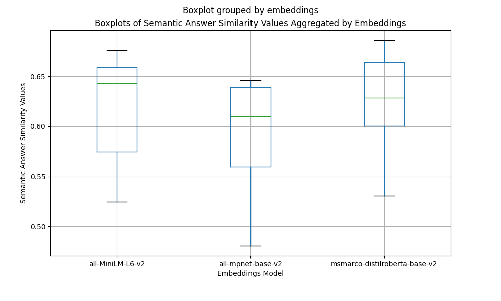
The box-plots above show that:
- The
all-MiniLM-L6-v2and themsmarco-distilroberta-base-v2embedding models outperform theall-mpnet-base-v2 - The
msmarco-distilroberta-base-v2scores have less variance, indicating that this model is more stable totop_kandchunk_sizeparameter variations than the other models - All three embedding models have an outlier corresponding to the highest-scoring and lowest-scoring parameter combination
- Not surprisingly, all the lowest scores outliers correspond to
top_k=1andchunk_size=64 - The highest scores outliers correspond to
top_k=3and achunk_sizeof128or256
Since we have the ground truth answers, we focuses on the Semantic Similarity Answer, but let’s also look at the Faithfulness and Context Relevance scores for a few examples. For that, we will need to load the detailed scores:
detailed_best_sas_df = pd.read_csv("results/aragog_results/detailed_all-MiniLM-L6-v2__top_k:3__chunk_size:128.csv")

def inspect(idx):
    print("Question: ")
    print(detailed_best_sas_df.loc[idx]['questions'])
    print("\nTrue Answer:")
    print(detailed_best_sas_df.loc[idx]['true_answers'])
    print()
    print("Generated Answer:")
    print(detailed_best_sas_df.loc[idx]['predicted_answers'])
    print()
    print(f"Context Relevance  : {detailed_best_sas_df.loc[idx]['context_relevance']}")
    print(f"Faithfulness       : {detailed_best_sas_df.loc[idx]['faithfulness']}")
    print(f"Semantic Similarity: {detailed_best_sas_df.loc[idx]['sas']}")
Let’s look at the query question 6:
inspect(6)
Question:
How does BERT's performance on the GLUE benchmark compare to previous state-of-the-art models?

True Answer:
BERT achieved new state-of-the-art on the GLUE benchmark (80.5%), surpassing the previous best models.

Generated Answer:
BERT's performance on the GLUE benchmark significantly outperforms previous state-of-the-art models, achieving 4.5% and 7.0% respective average accuracy improvement over the prior state of the art.

Context Relevance  : 1.0
Faithfulness       : 1.0
Semantic Similarity: 0.9051246047019958

Contexts:
recent work in this area.
Since its release, GLUE has been used as a testbed and showcase by the developers of several
influential models, including GPT (Radford et al., 2018) and BERT (Devlin et al., 2019). As shown
in Figure 1, progress on GLUE since its release has been striking. On GLUE, GPT and BERT
achieved scores of 72.8 and 80.2 respectively, relative to 66.5 for an ELMo-based model (Peters
et al., 2018) and 63.7 for the strongest baseline with no multitask learning or pretraining above the
word level. Recent models (Liu et al., 2019d; Yang et al., 2019) have clearly surpassed estimates of
non-expert human performance on GLUE (Nangia and Bowman, 2019). The success of these models
on GLUE has been driven by ever-increasing model capacity, compute power, and data quantity, as
well as innovations in
---------
56.0 75.1
BERT BASE 84.6/83.4 71.2 90.5 93.5 52.1 85.8 88.9 66.4 79.6
BERT LARGE 86.7/85.9 72.1 92.7 94.9 60.5 86.5 89.3 70.1 82.1
Table 1: GLUE Test results, scored by the evaluation server ( https://gluebenchmark.com/leaderboard ).
The number below each task denotes the number of training examples. The “Average” column is slightly different
than the official GLUE score, since we exclude the problematic WNLI set.8BERT and OpenAI GPT are single-
model, single task. F1 scores are reported for QQP and MRPC, Spearman correlations are reported for STS-B, and
accuracy scores are reported for the other tasks. We exclude entries that use BERT as one of their components.
We use a batch size of 32 and fine-tune for 3
epochs over the data for all GLUE tasks. For each
task, we selected the best fine-tuning learning rate
(among 5e-5,
---------
4e-5, 3e-5, and 2e-5) on the Dev set.
Additionally, for BERT LARGE we found that fine-
tuning was sometimes unstable on small datasets,
so we ran several random restarts and selected the
best model on the Dev set. With random restarts,
we use the same pre-trained checkpoint but per-
form different fine-tuning data shuffling and clas-
sifier layer initialization.9
Results are presented in Table 1. Both
BERT BASE and BERT LARGE outperform all sys-
tems on all tasks by a substantial margin, obtaining
4.5% and 7.0% respective average accuracy im-
provement over the prior state of the art. Note that
BERT BASE and OpenAI GPT are nearly identical
in terms of model architecture apart from the at-
tention masking. For the largest and most widely
reported GLUE task, MNLI, BERT obtains a 4.6%
absolute accuracy improvement. On the official
GLUE leaderboard10, BERT LARGE obtains a score
of
---------
In this example, the context relevancy and faithfulness scores are both 1.0. This indicates that the context is relevant to the question and our RAG LLM used this context to generate a semantically similar answer to the correct (ground-truth) answer.
Let’s take a look at another example:
inspect(44)
Question:
How should future language model benchmarks be structured to ensure a holistic assessment of models' capabilities and knowledge breadth?

True Answer:
Future benchmarks should integrate a broader spectrum of subjects and cognitive skills, emphasizing the inclusion of tasks that test models' ethical reasoning, understanding of human values, and ability to perform complex problem-solving, beyond the mere scale of data and parameters.

Generated Answer:
Future language model benchmarks should be structured to measure knowledge acquired during pretraining by evaluating models exclusively in zero-shot and few-shot settings across a diverse set of subjects that humans learn. The benchmark should cover a wide range of subjects across STEM, humanities, social sciences, and more, ranging in difficulty from elementary to advanced professional levels. It should test both world knowledge and problem-solving ability, ensuring a holistic assessment of models' capabilities and knowledge breadth.

Context Relevance  : 0.6
Faithfulness       : 1.0
Semantic Similarity: 0.6483339071273804

Contexts:
learning model
usage should be developed for guiding users to learn ‘Dos’
and Dont’ in AI. Detailed policies could also be proposed
to list all user’s responsibilities before the model access.
C. Language Models Beyond ChatGPT
The examination of ethical implications associated with
language models necessitates a comprehensive examina-
tion of the broader challenges that arise within the domainof language models, in light of recent advancements in
the field of artificial intelligence. The last decade has seen
a rapid evolution of AI techniques, characterized by an
exponential increase in the size and complexity of AI
models, and a concomitant scale-up of model parameters.
The scaling laws that govern the development of language
models,asdocumentedinrecentliterature[84,85],suggest
thatwecanexpecttoencounterevenmoreexpansivemod-
els that incorporate multiple modalities in the near future.
Efforts to integrate multiple modalities into a single model
are driven by the ultimate goal of realizing the concept of
foundation models [86].
---------
language models are
at learning and applying knowledge from many domains.
To bridge the gap between the wide-ranging knowledge that models see during pretraining and the
existing measures of success, we introduce a new benchmark for assessing models across a diverse
set of subjects that humans learn. We design the benchmark to measure knowledge acquired during
pretraining by evaluating models exclusively in zero-shot and few-shot settings. This makes the
benchmark more challenging and more similar to how we evaluate humans. The benchmark covers
57subjects across STEM, the humanities, the social sciences, and more. It ranges in difficulty from
an elementary level to an advanced professional level, and it tests both world knowledge and problem
solving ability. Subjects range from traditional areas, such as mathematics and history, to more
1arXiv:2009.03300v3 [cs.CY] 12 Jan 2021Published as a conference paper at
---------
a
lack of access to the benefits of these models for people
who speak different languages and can lead to biased or
unfairpredictionsaboutthosegroups[14,15].Toovercome
this, it is crucial to ensure that the training data contains
a substantial proportion of diverse, high-quality corpora
from various languages and cultures.
b) Robustness: Another major ethical consideration
in the design and implementation of language models is
their robustness. Robustness refers to a model’s ability
to maintain its performance when given input that is
semantically or syntactically different from the input it
was trained on.
Semantic Perturbation: Semantic perturbation is a type
of input that can cause a language model to fail [40, 41].
This input has different syntax but is semantically similar
to the input used for training the model. To address this,
it is crucial to ensure that the training data is diverse and
representative of the population it will
---------
It seems that for this question, the content is not completely relevant (Context Relevance = 0.6) and only the second context was used to generate the answer.
Running your own experiments
If you want to run this experiment yourself, follow the Python code
evaluation_aragog.py in the
haystack-evaluation repository.
Start by cloning the repository
git clone https://github.com/deepset-ai/haystack-evaluation
cd haystack-evaluation
cd evaluations
Next, run the Python script:
usage: evaluation_aragog.py [-h] --output_dir OUTPUT_DIR [--sample SAMPLE]
You can specify the output directory to hold the results and the sample size, i.e.: how many questions to use for the evaluation.
Don’t forget to define your Open AI API key in the environmental variable
OPENAI_API_KEY
OPENAI_API_KEY=<your_key> python evaluation_aragog.py --output-dir experiment_a --sample 10
Execution Time and Costs
NOTE: all the numbers reported were run on an Mac Book Pro Apple M3 Pro with 36GB of RAM with Haystack 2.2.1 and Python 3.9
Indexing
The Indexing pipeline needs to consider the parameter combinations defined below:
- 3 different values for
embedding_model - 3 different
chunk_sizevalues
Therefore, the index runs 9 times in total.
RAG Pipeline
The RAG pipeline needs to run 27 times, since the following parameters affect the retrieval process:
- 3 different values for
embedding_model - 3 different
top_kvalues - 3 different
chunk_sizevalues
This needs to run for each of the 107 questions, so in total, the RAG pipeline will run 2.889 times (3 x 3 x 3 x 107) and produce 2889 calls to OpenAI API.
Evaluation Pipeline
The Evaluation pipeline also runs 27 times since all parameter combinations need to be evaluated for each of the 107 questions. Note, however, that the Evaluation pipeline contains two Evaluators that rely on an LLM through OpenAI API, so this pipeline runs 2.889 times. However, due to the Faithfulness and ContextRelevance evaluators, it will produce 5.778 (2 x 2.889) calls to OpenAI API.
You can see the detailed running times for each parameter combination in the Benchmark Times Spreadsheet.
Pricing
For detailed pricing information, visit OpenAI Pricing 💸
Lessons Learned
In this article, we have shown how to use the Haystack Evaluators to find the best combination of parameters that yield the best performance of our RAG pipeline, as opposed to using only the default parameters.
For this ARAGOG dataset, in particular, the best performance is achieved using the msmarco-distilroberta-base-v2 embeddings model instead of the default model (sentence-transformers/all-mpnet-base-v2), together with a top_k=3 and a chunk_size=128.
A few learnings are important to take:
- When using an LLM through an external API, it is important to account for potential network errors or other issues. Ensure that during your experiments, running the questions through the RAG pipeline or evaluating the results doesn’t crash due to an error, for instance, by wrapping the call within a
try/exceptcode block. - Before starting your experiments, estimate the costs and time involved. If you plan to use an external LLM through an API, calculate approximately how many API calls you will need to run queries through your RAG pipeline and evaluate the results if you use LLM-based evaluators. This will help you understand the total costs and time required for your experiments.
- Depending on your dataset size and running time, Python notebooks might not be the best approach to run your experiments; a Python script is probably a more reliable solution.
- Beware of which parameters affect which components. For instance, for indexing, only the
embedding_modeland thechunk_sizeare important - this can reduce the number of experiments you need to carry out.
Explore a variety of evaluation examples tailored to different use cases and datasets by visiting the haystack-evaluation repository on GitHub.